A DC-DC converter can pass a room-temperature bench test and still oscillate after an output capacitor substitution or a change in customer load. When that happens, replacing compensation resistors at random makes the investigation difficult to reproduce. Start by identifying the instability, model the actual power stage, and adjust the loop with a measurable target.
This guide covers analog voltage-mode and current-mode buck and boost converters. It focuses on accessible error-amplifier compensation networks. Internally compensated devices require the manufacturer's approved component ranges; digital control and LLC resonant converters need different methods.
The practical objective is adequate stability margin across the operating range while meeting the load's voltage deviation and recovery requirements. A fast response at one operating point is insufficient evidence for a production release.
Identify the disturbance before changing compensation
Capture output voltage and inductor current together. Include input voltage, enable, or the controller's fault indication when a restart is involved. Record the load, temperature, probe arrangement, switching mode, and time scale. A repeating restart may be current-limit hiccup or input undervoltage rather than a small-signal loop oscillation.
Probe directly across the output capacitor with a short ground connection. A long probe ground lead can exaggerate switching spikes and send the investigation in the wrong direction. Repeat the capture with a shorter connection before changing components. If the apparent spike changes substantially while the load and converter settings remain fixed, the probing arrangement is influencing the result.
| Observed behavior | First checks | Appropriate next action |
|---|---|---|
| Low-frequency ringing after a load step | Loop gain, actual load slew rate, operating mode | Measure crossover and phase margin; inspect the full response |
| Alternating inductor-current peaks on successive switching cycles | Peak current-mode operation, duty ratio, slope compensation | Follow the controller's current-loop design procedure |
| Narrow spikes at switching edges | Probe ground, switch-node coupling, layout | Correct the measurement and noise paths before retuning |
| Repeated startup attempts | Input droop, current limit, soft start, load inrush | Capture the sequence and identify the protection trigger |
| Failure after a capacitor change | Effective capacitance, ESR versus frequency and temperature | Recalculate the power stage and repeat qualification |
| Light-load bursts | Burst mode, pulse skipping, CCM-to-DCM transition | Compare with specified controller behavior and load requirements |
Inspect inductor saturation and current-sense integrity before blaming the outer voltage loop. Saturation changes the current ramp and can trigger protection. Input-filter interaction also deserves attention when the converter behaves differently on a laboratory supply and on the customer's cable harness.
In peak current-mode control, inadequate slope compensation can produce subharmonic behavior above 50% duty ratio. This is a sampled current-loop problem; changing the outer error-amplifier RC network is not its primary cure. Many controllers provide an internal ramp, so check its specified limits before adding anything externally. Operation above 50% duty is normal when properly designed. Inspect successive switching cycles at a time scale that makes alternate peak heights visible. A slow output-voltage capture alone can hide this distinction.
Read loop gain rather than output gain
Crossover frequency, fc, is where the magnitude of the return ratio, or loop gain, reaches unity at 0 dB. It is not defined by the closed-loop output transfer function falling to 0 dB. Phase margin is the remaining phase separation from -180 degrees at that crossing, using the conventional negative-feedback phase convention.
A phase margin around 45 to 60 degrees is a common starting target, with roughly 10 dB gain margin where a relevant phase crossing exists. These are engineering targets, not a universal pass standard. Agree on acceptance limits before testing and retain allowance for component spread. A larger phase margin does not automatically mean a slower converter; bandwidth and the rest of the loop shape also matter. Record the operating point next to every margin result so that a change in load or input voltage cannot be mistaken for an improvement from the new compensation values.
Inspect for additional gain crossings. One attractive phase-margin number can hide a problematic high-frequency response. Transient results should support the frequency-domain result, especially when the converter enters a nonlinear mode during a large load change.

Choose compensation from the actual power stage
Type-I, Type-II, and Type-III describe transfer-function shapes. They do not define a universal pinout or interchangeable component values. A transconductance error amplifier and a voltage-output operational amplifier use different design equations.
| Compensation | Frequency-shaping elements | Typical use and limitation |
|---|---|---|
| Type-I | An integrator | Suitable when a sufficiently low crossover leaves adequate plant phase; often sacrifices response speed |
| Type-II | Integrator, one zero, one high-frequency pole | Common for current-mode bucks whose plant is approximately first order over the intended bandwidth |
| Type-III | Integrator, two zeros, two high-frequency poles | Often needed for voltage-mode bucks crossing above the LC resonance, especially with low-ESR capacitors |
A current-mode buck often permits Type-II because the inner current loop changes the low-frequency plant seen by the outer voltage loop. That approximation does not remove switching-related dynamics, current-loop limits, or the right-half-plane zero in a CCM boost converter.
Voltage mode does not always require Type-III. Type-II can work when the chosen crossover and available plant phase permit it, including appropriately low-bandwidth designs. The real question is how much phase lead is required around crossover. Type-II can add up to approximately 90 degrees of lead relative to its integrator baseline; Type-III can add up to approximately 180 degrees. Neither number is a guaranteed system phase margin. Before calculating values, identify whether the error amplifier delivers a voltage or a current and draw the exact external network. A formula for one implementation may give the wrong component values for another.
Calculate the frequencies that constrain the design
Use effective output capacitance at operating voltage and temperature. A nominal MLCC value can be substantially higher than its working capacitance. ESR also changes with frequency and temperature, so a mixed electrolytic and ceramic bank is not always represented adequately by one capacitance and one ESR. Build the initial model from the capacitor supplier's bias and temperature curves, then repeat the calculation at the lowest credible capacitance. The nominal value printed on the BOM is not enough.
For an idealized CCM buck, the LC resonant frequency is:
fLC = 1 / (2*pi*sqrt(L*Cout))
For a single lumped output capacitor model, the ESR zero is:
fESR = 1 / (2*pi*ESR*Cout)
The ESR zero is a left-half-plane zero: it raises gain slope and provides phase lead. It does not inherently cause phase lag. Replacing an electrolytic capacitor with low-ESR ceramics can remove useful phase lead near crossover, while changing the LC resonance. A compensator pole may be used to offset the ESR zero's gain rise, but placement must follow the complete loop response. Check both magnitude and phase after a capacitor substitution. An apparently improved ripple measurement does not prove that the feedback loop retains its previous stability margin.
For an ideal CCM boost with a resistive load, a useful first estimate is:
fRHPZ = Rload*(1-D)^2 / (2*pi*L)
Here D is duty ratio and Rload is Vout/Iout. This zero increases gain while adding phase lag. An ordinary compensation zero cannot safely cancel it. Evaluate its lowest frequency over the operating range and keep crossover well below it. A starting ceiling near one fifth of that frequency is common; the controller's design procedure takes priority. Increasing boost duty initially reduces the interval available to deliver inductor energy to the output. That inverse initial response is why the bandwidth must remain below this limit.
Consider an illustrative 12 V to 24 V boost at 2 A with a 22 microhenry inductor. Ignoring losses, D is 0.5 and Rload is 12 ohms, giving fRHPZ about 21.7 kHz. One fifth is only 4.3 kHz. Even with a 500 kHz switching frequency, choosing 50 kHz crossover from a switching-frequency rule would miss the dominant limit. Lower input voltage can tighten the constraint further.
For a buck without that RHP-zero constraint, fsw/10 can be a useful initial bandwidth estimate. Reduce it if plant phase, amplifier bandwidth, sampling effects, or the datasheet requires. Do not apply a blanket fsw/5 target to every controller.
Adjust RC values with a defined objective
Begin with the manufacturer's model and compensation equations for the exact controller. Include the feedback-divider gain, modulator or current-sense gain, amplifier characteristics, and actual L and C values. Calculate the gain needed at the proposed crossover, then position zeros and poles to provide the required phase shape.
Keep the COMP connection short and return its components to the specified signal ground. A correct RC calculation cannot compensate for noise coupled into a poorly routed feedback node.
For a common transconductance Type-II arrangement, a series Rcomp and Ccomp branch connects COMP to signal ground, with a smaller Chf capacitor in parallel with the whole branch. Its impedance has:
fz = 1 / (2*pi*Rcomp*Ccomp)
fp = (Ccomp + Chf) / (2*pi*Rcomp*Ccomp*Chf)
When Chf is much smaller than Ccomp, fp is approximately 1/(2*pi*Rcomp*Chf). These equations apply to this stated network only. They locate its zero and pole; they do not establish system crossover without the remaining loop gains.
For example, 10 kilohms, 10 nF, and 100 pF give fz about 1.59 kHz and fp about 161 kHz. Suppose measurements justify reducing compensation gain while preserving those frequencies. Scaling the resistor to 6.8 kilohms and both capacitors by 10/6.8 preserves the RC products and reduces the ideal network impedance by 0.68, about 3.35 dB. Select available values and recalculate. The crossover shift depends on the plant's slope and must be measured; these values are an arithmetic example, not a replacement BOM.
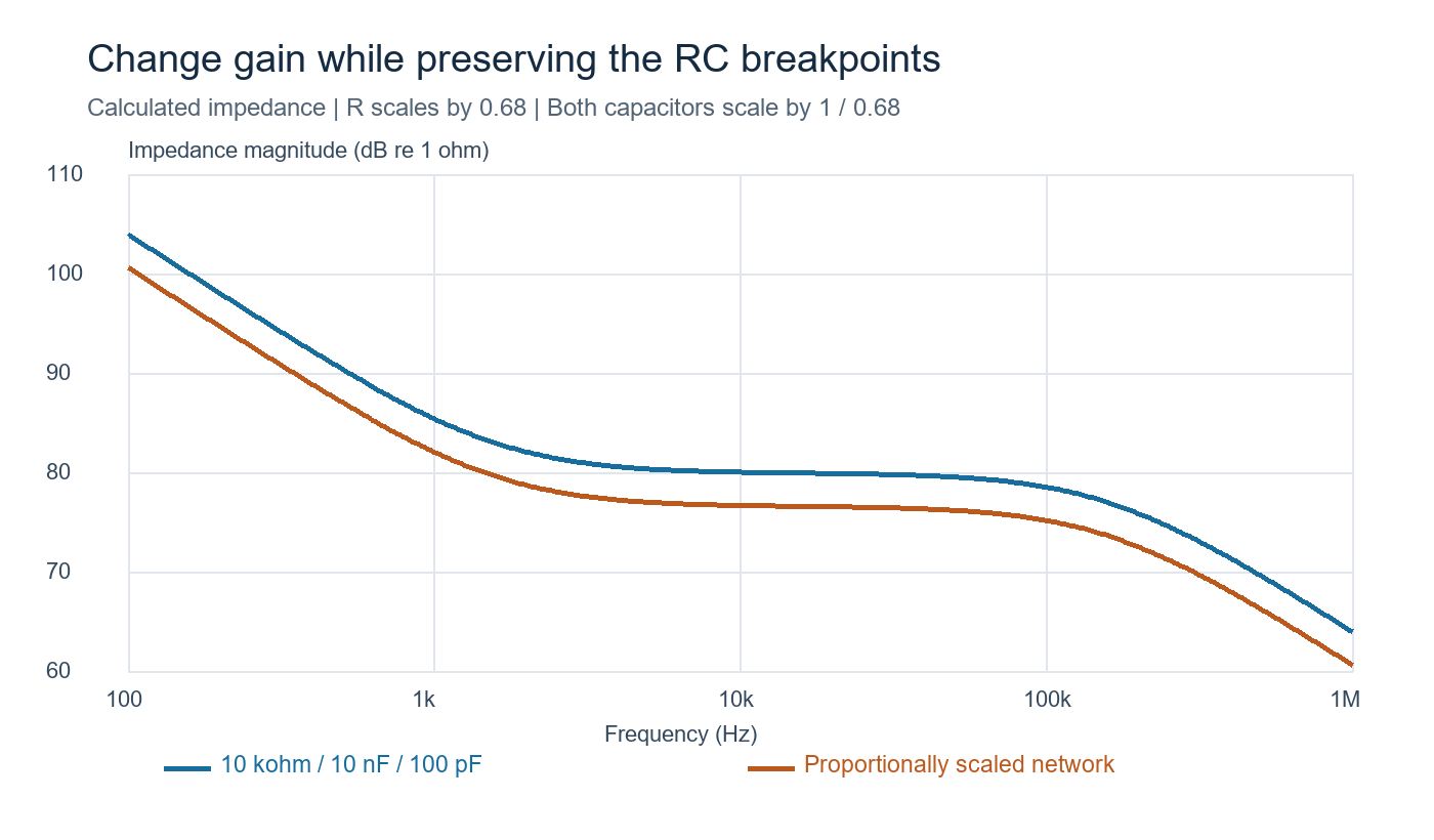
If phase margin is insufficient, reducing gain can move crossover to a more favorable region. If more phase lead is needed, adjust zero and pole separation around the intended crossover and recalculate the resulting gain. Moving one capacitor may change several features at once, so record the predicted effect before soldering.
To attenuate high-frequency gain sooner, a high-frequency pole generally moves downward, not upward. Moving it too close to crossover adds phase lag where it can hurt stability. This tradeoff is why a blanket instruction to increase or decrease a capacitor is unreliable.
For Type-III, place the two zeros to address the LC phase loss and choose the upper poles from the ESR behavior and high-frequency limits. Then solve the exact implementation's component equations. Avoid relying on perfect pole-zero cancellation across production tolerances.
Verify the board with frequency and time domain tests
Provide an injection point during PCB design where the required impedance conditions hold. A small resistor between the low-impedance output sense point and the upper feedback resistor is a common arrangement. Keep the DC feedback path intact and inject a small AC signal through a suitable transformer. Use the analyzer's documented channel ratio and phase convention.
Check that the perturbation is large enough for reliable measurement but small enough to avoid clipping, current limit, or mode changes. Repeat a sweep with a different injection amplitude: large changes in the measured result warrant investigation. Transformer bandwidth, probe loading, and instrument dynamic range matter. Select the injection transformer for the frequency range being measured and use short probe connections to a quiet reference. A sweep outside the usable measurement range cannot establish a reliable margin.
After each RC change, save the Bode plot and a load-step capture under the same conditions. Measure voltage excursion and settling time against the equipment specification. A 10% to 90% load step is useful when representative, but specify its slew rate and dwell time. Excessively fast cabling or fixture transients can dominate the initial spike before the feedback loop responds.
Without a frequency-response analyzer, load steps can identify poor damping and guide a provisional adjustment. They cannot uniquely determine phase margin. Some oscilloscopes support frequency-response measurements with the right stimulus and analysis options; a dedicated analyzer is not the only route. Check whether the available instrument can generate a swept stimulus, measure the two feedback signals, and calculate their complex ratio. A standard time-domain capture does not provide those functions by itself.
Startup needs its own test. Overshoot can involve soft-start tracking, amplifier saturation, prebiased outputs, minimum on-time, or insufficient discharge capability. Reducing low-frequency gain indiscriminately can worsen regulation without resolving the cause. Likewise, a waveform settling in two or three cycles is not a universal acceptance rule.
Qualify the settings for production
Keep the compensation components close to the controller and route feedback away from the switch node. Use the signal-ground connection recommended by the manufacturer. C0G or NP0 capacitors are useful for small compensation values; when their capacitance range is impractical, choose another dielectric using its actual bias, tolerance, and temperature data.
| Qualification condition | Evidence to retain | Release decision |
|---|---|---|
| Minimum and maximum input at representative loads | Loop plots, operating mode, current waveforms | Margins meet the agreed requirement |
| Cold and hot operation after thermal stabilization | Effective operating conditions and transient captures | No unexplained oscillation or protection entry |
| Light load and mode transitions | Burst or pulse-skipping behavior and output excursion | Behavior meets the load specification |
| Worst-case L, C, ESR and approved alternatives | Model corners and measurements on representative builds | Substitutions retain acceptable response |
| Startup, shutdown and load release | Peak voltage, recovery, prebias behavior where applicable | No violation of equipment limits |
| Actual cables, input filter and customer load | System-level voltage and current captures | Bench conclusions hold in the application |
Engineering qualification should cover these corners; every production unit does not necessarily need a full frequency sweep. Define routine screening from the observed failure modes and retain a traceable compensation revision, PCB revision, and approved BOM. Repeat the relevant qualification when inductors, capacitors, controller variants, or operating limits change.
For equipment buyers, request test conditions alongside any stability claim. A single full-load room-temperature plot says little about a cold startup or a different output capacitor bank. When discussing a SIPURUI power supply for your equipment, share the input range, load-step profile, ambient conditions, and external capacitance so the application requirements are explicit.
Effective compensation tuning ends with a reproducible design record: an identified failure mechanism, calculated component changes, and measured performance across the intended operating range.