Build a practical switching power supply burn-in program, distinguish MTBF from service life, plan accelerated testing, and report reliability claims with defensible statistics.
Overview
A switching power supply can pass every bench check and still fail after a few days in the field. The usual gap is not basic function. It is time, temperature, component variation, and workmanship.
Burn-in testing is designed to expose early failures before a unit ships. MTBF analysis answers a different question: how frequently failures are expected across a population under stated conditions. Neither test tells you the exact service life of one power supply, and neither can compensate for weak thermal design or poor component derating.
This guide lays out a practical reliability workflow for AC-DC power supplies and DC-DC modules, from pre-test inspection through burn-in, accelerated life testing, statistical interpretation, failure analysis, and the final report.
Burn-in, MTBF, accelerated life, and service life are not interchangeable
These terms are often bundled together in supplier discussions, which is where many reliability claims go off track.
| Term | What it measures | What it does not prove |
|---|---|---|
| Burn-in | Screens for early failures and workmanship defects by operating units under controlled stress | The exact lifetime of a unit or a statistically defensible MTBF by itself |
| MTBF | A population-level estimate of time between failures, normally under a stated model and operating environment | Warranty period, wear-out life, or a promise that one unit will run for the quoted number of hours |
| Accelerated life test (ALT) | Uses elevated stress to obtain failures sooner, then relates test conditions to use conditions through a justified model | Valid results when the stress creates a different failure mechanism |
| Service life | Time until the product reaches an end-of-life criterion in its real application | The same value as a handbook MTBF prediction |
For non-repairable modules, mean time to failure (MTTF) is the more precise term. Power supply vendors nevertheless use MTBF widely, even when failed units are replaced rather than repaired. The important point is to define the metric, model, environment, duty cycle, and confidence level.
What a power supply burn-in test should accomplish
A useful burn-in program aims at the front end of the reliability curve, where latent manufacturing defects tend to appear. It can reveal marginal solder joints, damaged components, PCB cracks, insulation defects, unstable control loops, poor thermal interfaces, and parts that were already weak when assembled.
Burn-in also gives engineers time-series data. Output voltage may remain within tolerance while ripple rises, an optocoupler drifts, or a hotspot moves closer to a component limit. A pass/fail lamp will miss those changes.
Burn-in is a screen, not a repair process. A good unit does not become “more reliable” because it has accumulated hours in a chamber. Excessive temperature, voltage, or duration can consume useful life or introduce damage that the intended application would never create.

Choose the test condition from the objective
There is no universal burn-in recipe. A four-hour production screen and a 1,000-hour accelerated test serve different decisions and should not share the same stress profile.
| Test type | Typical starting condition | What to monitor | Best use |
|---|---|---|---|
| Ambient production burn-in | 25°C ± 5°C, rated input, 75-100% load, 4-24 h | Output voltage, current, ripple, case temperature, restart events | Screening workmanship and early component defects |
| Elevated-temperature burn-in | 45-60°C, rated input, full rated load, 24-72 h | Output drift, component temperatures, protection behavior, abnormal sound or odor | Design verification and thermal-margin checks |
| Dynamic-load endurance | 40-55°C with a defined load profile, such as 10-50-100-50% | Transient deviation, recovery time, oscillation, shutdown or reset | Industrial loads with cycling actuators, radios, motors, or processors |
| Input-voltage cycling | Minimum, nominal, and maximum specified input at a representative load | Start-up, hold-up, UVLO/OVP behavior, output interruption | Wide-input AC-DC supplies and DC-DC modules |
| Temperature cycling while powered | Product-specific low/high limits with controlled ramps and dwell periods | Intermittent faults, solder and connector behavior, cold start, hot restart | Equipment exposed to daily or seasonal temperature swings |
| Accelerated life test | Multiple stress cells, sample groups, and hundreds to thousands of hours | Individual failure times and failure modes | Estimating model parameters or demonstrating a reliability target |
Treat these as planning ranges, not standards. The product specification, applicable safety requirements, customer profile, component ratings, and intended environment must control the final plan.
A practical burn-in workflow
Freeze the sample identity and acceptance limits
Record the serial number, hardware revision, BOM revision, firmware if applicable, transformer lot, and any process deviations. Define the electrical and physical failure criteria before the chamber starts. If the team decides after the test which changes “count,” the data will be biased.
The pre-test check should cover the full input range at no load and at representative loads. Measure output regulation, ripple and noise with a documented probe method, start-up behavior, protection functions, and key component temperatures. For offline supplies, complete the relevant insulation-resistance, dielectric-withstand, earth-bond, and leakage-current checks using approved safety procedures.
Build the station around controlled stress and automatic logging
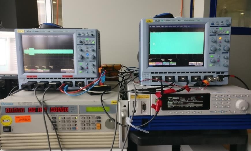
Use a programmable AC source or DC source with suitable protection, an electronic load with adequate voltage/current/power range, an oscilloscope for waveform checks, and a multichannel data acquisition system. Electronic loads are valuable because they can reproduce constant-current, constant-resistance, constant-power, and dynamic profiles that a fixed resistor cannot.
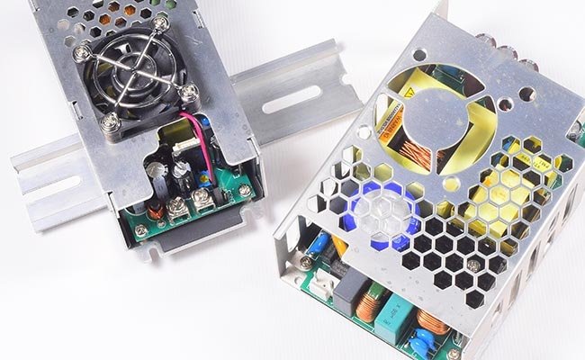
Place units so airflow is repeatable. Do not stack open-frame supplies or allow one unit's exhaust to heat the next. Thermocouples should be attached consistently to the same components: primary MOSFET case, transformer winding or accessible surface, rectifier, output inductor, and electrolytic capacitor can. Record chamber air temperature close to the units, not only the chamber controller reading.
Log input voltage, input current or power, output voltage, load current, and selected temperatures at a useful interval. Five to fifteen minutes is adequate for slow drift; transient tests require much faster acquisition. Add independent overtemperature, overcurrent, and smoke/fire protection appropriate to the energy involved.
Ramp into the operating point
Start under controlled conditions, confirm stable output, then raise load and chamber temperature according to the test plan. A cold unit taken directly to a high-temperature full-load condition adds a thermal shock that may not represent the intended test.
During the run, watch for more than loss of output. Flag repeated start attempts, audible changes, sudden temperature slope changes, increased ripple, output overshoot, fan anomalies, and protection events. For dynamic profiles, retain the programmed waveform and revision-controlled script with the report.
Cool down and repeat the electrical test
The post-test inspection is not optional. Disconnect the load, power down safely, and allow the sample to return to the defined room-temperature condition. Repeat the same electrical measurements used before burn-in, with the same instruments and probe arrangement.
Compare the results, not just the final pass/fail status. A unit may still regulate while its ripple has doubled or its overcurrent threshold has shifted close to the specification limit. Inspect electrolytic capacitors, adhesive, insulation, connectors, solder joints, PCB discoloration, and heat-damaged sleeving.
Apply pre-agreed failure criteria
A sample should normally be classified as failed if it shows any of the following:
no output, failure to start, or an unintended restart;
output voltage, ripple, transient response, or efficiency outside the product specification;
missing protection, nuisance protection, or a protection threshold outside its allowed range;
intermittent behavior that cannot be reproduced reliably after the test;
physical damage, leakage, bulging, charring, cracked insulation, or a damaged connector;
parameter drift beyond the defined acceptance limit, even if the unit still functions.
Temperature drift within the documented specification is not automatically a failure. It is still worth trending, especially when the same direction appears across a sample group.
MTBF prediction from the design
A parts-count or parts-stress prediction estimates system failure rate from component models. MIL-HDBK-217 remains a recognized framework for electronic reliability prediction, and other programs may specify Telcordia SR-332, IEC TR 62380-based methods, FIDES, or an organization-specific database.
For a simple series reliability model with a constant failure rate:
λsystem = Σ λi
MTBF = 1 / λsystem
The component failure rate is adjusted for factors such as part type, junction or ambient temperature, electrical stress, quality level, and environment. The result is useful for comparing design alternatives and checking whether the selected parts and derating policy support a target.
It remains a prediction. It does not include every workmanship defect, supplier excursion, PCB contamination issue, transformer winding error, or application-specific transient. State the method, revision, environment category, assumed temperatures, duty cycle, and whether the result is a point estimate or includes uncertainty.
MTBF demonstration with accelerated testing
ALT is useful when a normal-use test would require impractical calendar time. The test increases a relevant stress, measures failures, and uses a physical or empirical relationship to translate the exposure back to use conditions.
For temperature-driven mechanisms, an Arrhenius model is often considered:
AF = exp[(Ea / k) × (1 / Tuse - 1 / Tstress)]
where AF is the acceleration factor, Ea is activation energy in electron-volts, k is Boltzmann's constant (8.617 × 10^-5 eV/K), and both temperatures are in kelvin.
Using Ea = 0.70 eV purely as an example, a test at 80°C compared with a 40°C use condition gives an acceleration factor of about 18.7. One hundred test hours would then contribute about 1,870 equivalent device-hours for that temperature-driven mechanism. A different activation energy produces a different answer, and the model says nothing about failure modes that temperature does not accelerate in the same way.
The failure mechanism must remain the same
An ALT becomes misleading when the stress creates a new mechanism. Running an 85°C-rated electrolytic capacitor with a core temperature above its rating, exceeding semiconductor junction limits, or applying unrealistic overvoltage may produce fast failures that would not occur in service.
Temperature is also not a universal accelerator. Solder fatigue may require thermal cycling; insulation degradation may depend on voltage, humidity, and contamination; mechanical connector faults may respond to vibration; and control-loop instability may appear only under a specific load transition.
Use total equivalent device-hours and report confidence
For an exponential constant-failure-rate model, total equivalent exposure is the sum of each sample's test time multiplied by the justified acceleration factor for its stress cell.
With zero observed failures, a one-sided lower confidence bound for MTBF is:
MTBF lower bound = Teq / [-ln(1 - C)]
where Teq is total equivalent device-hours and C is the confidence level.
Suppose 20 units each complete 1,000 hours and the justified acceleration factor is 10. Total equivalent exposure is 200,000 device-hours. With zero failures, the MTBF lower bound is approximately 218,300 hours at 60% confidence, but only 86,900 hours at 90% confidence. The same test data supports different claims depending on the required confidence.
If failures occur, retain the exact failure times and account for suspended units. A Weibull or other life distribution may be more appropriate than the exponential model when the failure rate changes with time. Reliability specialists should define the analysis before the test, not after seeing the data.
| Validation purpose | Sensible planning approach | Required output |
|---|---|---|
| Engineering screen | Small pilot group at one controlled elevated condition | Failure observations, drift trends, thermal margin, and design actions; avoid a strong MTBF claim |
| Reliability demonstration | Sample size and duration calculated from target MTBF, confidence, allowed failures, and acceleration factor | Total/equivalent device-hours, failures, confidence bound, and model assumptions |
| Life-model development | Multiple stress levels with enough failures to fit the model | Distribution parameters, acceleration relationship, confidence intervals, and failure-mode consistency |
This approach is more defensible than specifying “15 units for 1,000 hours” without linking the plan to a target and confidence level.
MTBF is not the same as useful life
MTBF is frequently much larger than expected service life. There is no contradiction. A constant-rate MTBF describes failure frequency across a population in the useful-life region. Wear-out life asks when aging causes performance to cross an end-of-life criterion.
In a switching power supply, aluminum electrolytic capacitors often deserve special attention because electrolyte loss raises ESR and reduces capacitance. Capacitor manufacturers base lifetime estimates on the individual series, hot-spot temperature, ripple current, applied voltage, and mounting conditions. The familiar “life doubles for every 10°C reduction” is a useful approximation only within the range and conditions stated by the manufacturer; it is not a blanket rule for the entire power supply.
Do not publish an assumed 10,000- or 50,000-hour product life without a thermal model and component-specific calculation. Measure capacitor temperature in the assembled power supply, include ripple-current self-heating, and use the selected capacitor's data rather than a generic category value.
Common failures and what they usually point to
| Observation | Likely areas to investigate | Engineering response |
|---|---|---|
| Ripple rises gradually during hot operation | Output capacitor ESR/capacitance, rectifier heating, solder resistance, control-loop drift | Measure capacitor core/case temperature, review ripple current, inspect joints, and repeat loop-stability checks hot and cold |
| MOSFET fails after several hours at full load | Drain overshoot, avalanche energy, inadequate gate drive, thermal interface, transformer leakage inductance | Capture worst-case waveforms, review voltage and SOA margin, improve clamp/snubber and heat flow |
| Intermittent restart at light or changing load | Control-loop margin, burst-mode transition, auxiliary supply, optocoupler CTR spread | Test across line/load/temperature corners and verify compensation with component tolerances |
| A few units fail early while the rest remain stable | Workmanship, supplier variation, handling damage, contamination, marginal insulation | Perform failure analysis by serial/lot, audit process data, and improve incoming or production screening |
| Capacitor vents or bulges during ALT | Excess core temperature, ripple current, reverse or overvoltage stress, invalid acceleration condition | Stop the test, confirm ratings and thermocouple placement, then redesign the stress plan |
Seven mistakes that weaken a reliability program
Using room-temperature full-load operation as the only stress. It may miss hot optocoupler drift, capacitor heating, poor airflow, and load-dependent instability.
Applying ALT conditions to every production unit. A life-test stress can consume margin or create damage when used as a routine screen.
Checking only whether output is present. Drift, ripple, protection thresholds, and intermittent restarts matter.
Changing measurement methods between pre- and post-test. Different probes, bandwidth limits, cable lengths, or thermocouple positions can look like product drift.
Claiming MTBF from a tiny zero-failure run. The total exposure and confidence bound may be far below the marketing number.
Treating predicted MTBF as field evidence. A component model cannot see factory contamination, transformer workmanship, or application transients.
Ignoring failure-mode consistency in ALT. A fast failure is useful only when it represents a mechanism relevant to service.
Suggested programs for three product classes
For a cost-sensitive commercial supply, begin with a short production screen at rated input and a load that produces representative internal heating. Use sampling audits to confirm that the screen continues to catch the intended defects. A handbook prediction may support internal comparison, but the public specification should state its method and conditions.
For an industrial control supply, add elevated-temperature full-load operation, dynamic load profiles, line-voltage corners, powered temperature cycling, and hot/cold restart checks. A pilot ALT can identify weak components and help plan a later demonstration, but it should be reported as an engineering evaluation unless the sample size and statistics support more.
For a high-reliability supply, build the plan from a reliability requirement and mission profile. Use multiple samples and stress cells where necessary, independent test monitoring, calibrated instrumentation, a pre-approved statistical analysis, and formal failure analysis. Reliability growth requires redesign and retest; accumulating chamber hours alone is not a closure process.
What belongs in the final reliability report
The report should allow another engineer to reconstruct both the exposure and the conclusion. Include:
product identification, serial numbers, hardware/BOM revisions, and sample selection method;
test objective, applicable requirements, planned stresses, duration, and acceptance criteria;
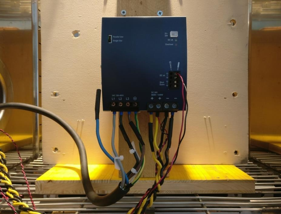
chamber, source, load, measurement equipment, calibration status, wiring, airflow, and sensor locations;
pre-test data, continuous logs, anomalies, operator interventions, and post-test data;
every failure time, symptom, failure definition, censoring rule, and failure-analysis result;
MTBF prediction method or test model, acceleration factors, equivalent device-hours, confidence level, and limitations;
corrective actions, ownership, verification status, and the exact conclusion supported by the data.
Reliability is designed in, then verified
Burn-in has a narrow but valuable job: find early defects and reveal performance drift under controlled operation. MTBF prediction helps compare designs. Accelerated testing can support a population-level reliability claim when the stress model, sample exposure, failure data, and confidence calculation are defensible.
The strongest program connects all three to field conditions. Component derating, thermal design, loop stability, transformer construction, PCB cleanliness, and process control create reliability. Testing shows whether those decisions hold up.
For OEM projects, SIPURUI can align an AC-DC or DC-DC power supply test plan with the input range, cabinet temperature, load profile, and reporting requirements of the target equipment. The useful conversation starts with the application and acceptance criteria, not with a headline MTBF number.